
The 3-D Utility Function
To build portfolios that are truly tailored to an individual’s risk profile, one must account for all three of the primary risk preferences expressed by humans: risk aversion, loss aversion, and reflection. In what follows we begin by reviewing how portfolios can be constructed from a utility function. We then show how one can easily extend the classic mean-variance approach, solely focused on risk aversion, to a more realistic 3-D risk preference paradigm, which additionally incorporates loss aversion and reflection.
What is Expected Utility Optimization?
To find the ideal investment portfolio for a human being we must calculate the expected utility (EU) for every possible portfolio, i.e. combination of assets, and choose the portfolio with the highest EU. In this framework, the EU for a single portfolio is defined as:
Equation 1 Portfolio Expected Utility
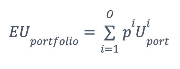
where we sum over all O possible portfolio utility outcomes Uporti over the next time period (we use one-month forward-looking steps here), each with probability pi, and where an outcome is defined as the joint return outcome of all assets during the next month.
Let’s for the moment assume our client’s utility function is the power utility function:
Equation 2 Power Utility
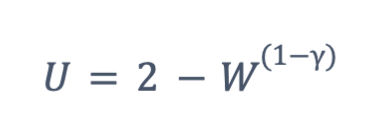
where W is the one-month wealth change 1 + rp, rp is the one-month period portfolio return, and γ is risk aversion (parameterized between 1.5 and 12).
In Table 1 we do a simple brute force EU optimization for two different portfolios and three possible outcomes, to keep things simple. We first calculate the utility of each portfolio in each outcome, and then find the average across all outcomes for each portfolio. The expected utility of Portfolio 1 is greater than the expected utility of Portfolio 2, making Portfolio 1 the optimal solution. Of course, in practice, we would deploy an optimizer so we could choose amongst all possible portfolios and incorporate a much larger number of potential outcomes.
Table Brute Force EU Optimization; Assumes γ = 3.
Portfolio 1: Stock 75%, Bonds 25%

Portfolio 2: Stock 60%, Bonds 40%

Now it turns out that a simpler problem to solve, mean-variance optimization, is a terrific approximation to the problem we just solved, which is precisely how Modern Portfolio Theory and its return vs. volatility paradigm became so popular. But this function has no information on loss aversion or reflection, key risk preference dimensions discovered in the 1970s. This function also has no information on skew or higher moments, a deficit increasingly of relevance in today’s markets.
What is a 3-D Utility Function?
Kahneman and Tversky introduced us to Prospect Theory in 1979, a key advancement in our understanding of decision making under uncertainty. This theory of human behavior introduced two new features of decision making to the classical theory encapsulated by the Power utility function.
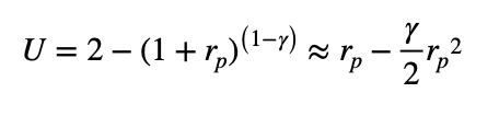
We could approximate Equation 2 very closely by:
Equation 3 Power Utility Approximated by a Quadratic Utility
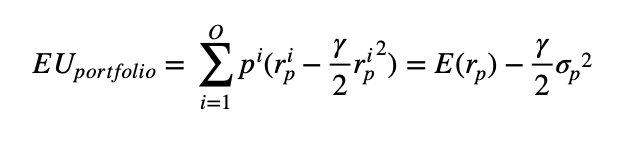
When we then go to find the EU of the portfolio with this utility function we find the classic mean-variance result:
Equation 4 Mean-Variance Approximation to EU when Using Power Utility
- Loss Aversion – the pain of losses is disproportionately greater than the pleasure of gains. The more loss aversion one has, the more unwilling they will be to play a game with very favorable terms if there is a possibility of losing even small amounts.
- Reflection – investors are risk averse in the gain domain but risk-seeking in the loss domain. We “hope to avoid losses” (risk-seeking in the loss domain) while being “afraid of missing gains” (risk-averse in the gain domain).
Incorporation of these two new dimensions of risk preferences in client portfolios is as simple as just inputting the refined utility function into Equation 1. And now a mean-variance approximation is no longer a good approximation for client utility, while simultaneously addressing the lack of higher moments that are much more present in today’s markets. The formula for this updated utility function gets a bit crazy, so its best to just to show how each preference updates the power utility function.
Figure 1 Moving from a 1D to 3D Utility Function

Figure 1 highlights how loss aversion generally pushes investors into portfolios with less volatility and less negative skew, since losses are so despised. We also see how reflection can lead to riskier portfolios, as the utility functions is curved upward in the loss regime, and will generally push portfolios in the opposite “risk” direction as loss aversion.
Parting Words
We now know, after decades of behavioral research advances, that human beings are not defined by a single risk parameter. By extending risk profiling to the two additional risk preference dimensions of loss aversion and reflection, portfolios have a much better shot at more accurately representing a client’s risk profile, while simultaneously accounting for higher order moments that are now omnipresent in today’s markets.
Leave a Reply